旋转位置编码的发展

Wed Jan 10 2024

# 前言

旋转位置编码（RoPE）目前已被广泛应用于主流大模型中，但是其存在外推性差的缺点，即在模型遇到输入长度超过训练长度时，模型性能会急剧下降。为了解决这个问题，出现了多个方法，如线性插值、NTK-Aware插值、NTK-by-parts、Dynamic NTK、YaRN。

关于RoPE原理，参考这篇文章：RoPE。

# 直接外推

在介绍大模型长度扩展方法之前，需要先说明一下直接外推为什么走不通。

在position interpolation (opens new window)的论文里提到，如果使用长文本从头训练模型，需要大量资源，不太现实。如果直接在预训练的模型上使用长文本微调，经过实验发现，微调超过10000个batches，有效长度从2048到256，效率较低。

现阶段已经存在一些技术可以使模型具有弱外推性，如RoPE。如果在RoPE上直接外推，扩展到模型之前没见过的文本长度，模型的困惑度会飙升到非常高的值（超过1000，正常是个位数）。

# 大模型长度扩展方法

以下将介绍几个主要的扩展方法。

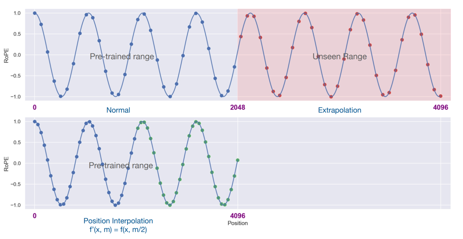
# Position Interpolation

上面提到了直接外推的缺点，后续position interpolation (opens new window)论文提出了位置插值方法。

我们定义函数 $f$ 为RoPE的方法，加入了位置插值的新方法为 $f'$ ，令 $x$ 为嵌入向量， $m$ 为位置下标。

$f'(x,m)=f(x,\frac{mL}{L'})$

其中 $L$ 表示原本的文本长度， $L'$ 表示更长的文本长度。它的意思是将更大的窗口范围从 $[0,L')$ 缩小到 $[0,L)$ 使其适应原始的窗口范围，每个位置的旋转弧度也相应缩小了。因为旋转弧度使线性变化的，所以也被称为线性插值。

position interpolation

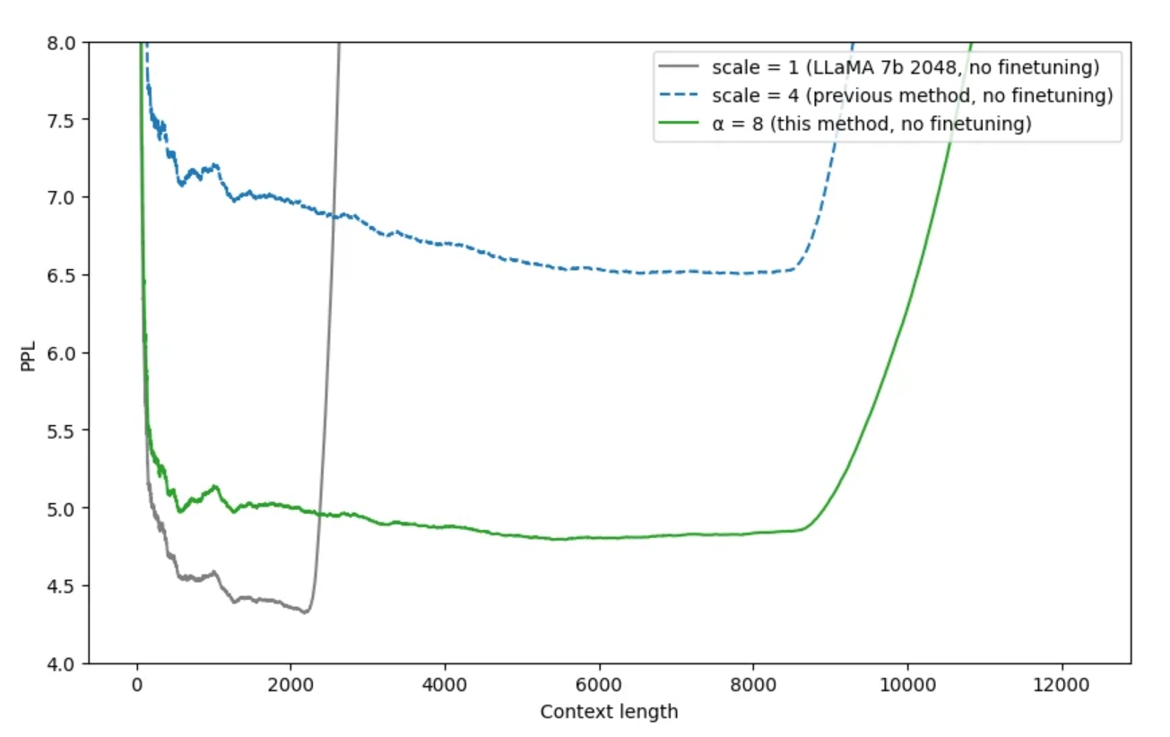
# NTK-Aware Interpolation

在PI出来后不久，有网友在reddit (opens new window)上发表了NTK-Aware插值方法。

作者表示无需微调即可扩展到8K+，同时使困惑度更低。作者受NTK启发，发现只使用位置插值，模型会更难识别接近的token的顺序和位置。因为在相同的区间内，被塞入了更多的token。

所以，作者设计了非线性方法，改变了RoPE中的base。

$b'=b*\alpha^{\frac{d}{d-2}}$

$m\theta_i=m(b')^{\frac{-2i}{d}}=m*(b*\alpha^{\frac{d}{d-2}})^{\frac{-2i}{d}}=m*b^{\frac{-2i}{d}}*\alpha^{\frac{-2i}{d-2}}$

其中 $\alpha^{\frac{-2i}{d-2}}$ 表示缩放因子，可以发现当位置为0时，公式会退化到原始的RoPE公式。随着位置从近到远，缩放因子逐渐变小，旋转弧度的变小速度变大。也就是说，前面的位置靠外推，后面的位置靠位置插值。

ntk-aware interpolation

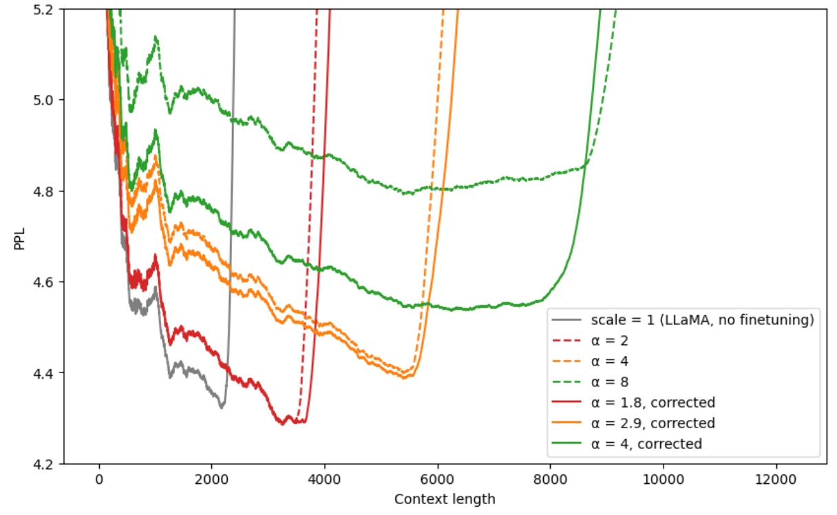
# NTK-by-parts Interpolation

在NTK-Aware Interpolation发布后一个月，作者又发表了优化版本NTK-by-parts Interpolation (opens new window)，困惑度再次降低。作者首先删除了缩放因子 $\alpha$ ，原因是这个超参数的值在不同大语言模型下不统一。新算法综合了位置插值、NTK-Aware插值和直接外推，分段采用不同的算法，这也是"by-parts"的含义。简单来说，在位置的前半段使用外推，后半段使用插值。前半段使用外推的原因是之前的算法使用插值导致性能有所下降。

接下来分析一下源码。

#Interpolation constants found experimentally for LLaMA (might not be totally optimal though)
#Do not change unless there is a good reason for doing so!
beta_0 = 1.25
beta_1 = 0.75
gamma_0 = 16
gamma_1 = 2

新算法引入了4个新的超参数，含义分别是两组周期个数的边界值。三角函数的周期是 $t=\frac{2\pi}{\theta}$ ，在窗口长度为 $L$ 的条件下的周期个数是 $n=\frac{L\theta}{2\pi}$ 。周期个数越大，表示位置越靠前，反之越靠后。所以代码中的gamma可以理解为表示前半段，beta表示后半段。因为频率越高，周期个数越大。

#Three RoPE extrapolation/interpolation methods
inv_freq_base = 1.0 / (base ** (torch.arange(0, dim, 2).float().to(device) / dim))
inv_freq_linear = 1.0 / (scale * (base ** (torch.arange(0, dim, 2).float().to(device) / dim)))
inv_freq_ntk = 1.0 / (find_newbase_ntk(dim, base, scale) ** (torch.arange(0, dim, 2).float().to(device) / dim))

定义了3个频率，分别是原始的RePE，线性插值和ntk-aware插值，接下来会用到。

def find_correction_factor(num_rotations, dim, base=10000, max_position_embeddings=2048):
    """反向求解位置下标"""
    return (dim * math.log(max_position_embeddings/(num_rotations * 2 * math.pi)))/(2 * math.log(base)) #Inverse dim formula to find number of rotations

def find_correction_range(low_rot, high_rot, dim, base=10000, max_position_embeddings=2048):
    """计算区间边界下标"""
    low = math.floor(find_correction_factor(low_rot, dim, base, max_position_embeddings))
    high = math.ceil(find_correction_factor(high_rot, dim, base, max_position_embeddings))
    return max(low, 0), min(high, dim-1) #Clamp values just in case

def linear_ramp_mask(min, max, dim):
    """频率系数归一化"""
    if min == max:
        max += 0.001 #Prevent singularity

    linear_func = (torch.arange(dim, dtype=torch.float32) - min) / (max - min)
    ramp_func = torch.clamp(linear_func, 0, 1)
    return ramp_func

#Combine NTK and Linear
low, high = find_correction_range(beta_0, beta_1, dim, base, original_max_position_embeddings)
inv_freq_mask = (1 - linear_ramp_mask(low, high, dim // 2).type(current_dtype).to(current_device)) * ntk_factor
inv_freq = inv_freq_linear * (1 - inv_freq_mask) + inv_freq_ntk * inv_freq_mask

这段代码计算了后半段位置的频率，find_correction_range返回了这段位置的边界下标，inv_freq_mask表示屏蔽系数经过归一化，最后的频率通过结合线性插值和ntk插值得出。

位置下标的公式推导：

$t=\frac{2\pi}{\theta}$

$n=\frac{L}{t}$

$n=\frac{L\theta}{2\pi}=\frac{Lb^{\frac{-2i}{d}}}{2\pi}$

$i=\frac{dlog\frac{L}{2n\pi}}{2logb}$

#Combine Extrapolation and NTK and Linear
low, high = find_correction_range(gamma_0, gamma_1, dim, base, original_max_position_embeddings)
inv_freq_mask = (1 - linear_ramp_mask(low, high, dim // 2).type(current_dtype).to(current_device)) * extrapolation_factor
inv_freq = inv_freq * (1 - inv_freq_mask) + inv_freq_base * inv_freq_mask

这段代码计算了前半段位置的频率，最后的频率通过结合上一段代码的频率和直接外推得出。

由上面代码可以得出，位置从近到远，依次使用外推（保持不变），ntk插值和线性插值。

ntk-by-parts interpolation

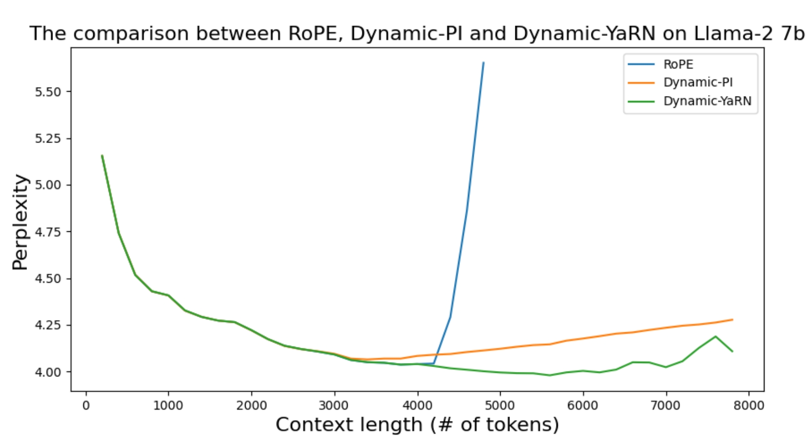
# Dynamic NTK Interpolation

同样是reddit的网友，受NTK-Aware启发，发表了Dynamic NTK Interpolation (opens new window)。作者表示线性插值和NTK插值都存在同样的问题，在训练长度内的表现都不如原始方法，而且NTK的方法存在写死的超参数 $\alpha$ ，有没有办法使 $\alpha$ 动态生成？作者提出如果推理长度在训练长度内不做插值，超过训练长度则每一步使用NTK插值动态放大base，并引入了新的超参数 $\alpha'$ 。

令 $l$ 为当前文本长度， $L$ 为训练最大长度，每生成一个token， $l$ 都会加1。

$\alpha'=\frac{\alpha*l}{L} - (\alpha - 1)$

dynamic ntk interpolation

# YaRN

NTK-Aware插值的后继者YaRN (opens new window)。YaRN是Yet another RoPE extensioN method的缩写。论文中详细讲述了线性插值、NTK-Aware插值、NTK-by-parts插值和Dynamic NTK插值的背景、起源和理由，非常值得一读。最后提出结合NTK-by-parts和温度系数t，得到了YaRN。

YaRN修改了注意力计算公式：

$softmax(\frac{q^T_mk_n}{t\sqrt{D}})$

关于温度系数t，其中 $s$ 是NTK的缩放因子， $l'$ 是当前长度，L是训练最大长度：

$\sqrt{\frac{1}{t}}=0.1*ln(s) + 1$

$s=max(1, \frac{l'}{L})$

def get_mscale(scale=1):
    if scale <= 1:
        return 1.0
    return 0.1 * math.log(scale) + 1.0

def forward(self, x, seq_len=None):
    # x: [bs, num_attention_heads, seq_len, head_size]
    # This `if` block is unlikely to be run after we build sin/cos in `__init__`. Keep the logic here just in case.
    if seq_len > self.max_seq_len_cached:
        self.max_seq_len_cached = seq_len

        self.yarn(seq_len / self.original_max_position_embeddings, x.device)

        t = torch.arange(self.max_seq_len_cached, device=x.device, dtype=self.inv_freq.dtype)
        freqs = torch.einsum("i,j->ij", t, self.inv_freq)
        # Different from paper, but it uses a different permutation in order to obtain the same calculation
        emb = torch.cat((freqs, freqs), dim=-1).to(x.device)

        self.register_buffer("cos_cached", (emb.cos() * self.mscale)[None, None, :, :].to(x.dtype), persistent=False)
        self.register_buffer("sin_cached", (emb.sin() * self.mscale)[None, None, :, :].to(x.dtype), persistent=False)
    return (
        self.cos_cached[:, :, :seq_len, ...].to(dtype=x.dtype),
        self.sin_cached[:, :, :seq_len, ...].to(dtype=x.dtype),
    )

def yarn(self, scale, device):
    pos_freqs = self.base ** (torch.arange(0, self.dim, 2).float().to(device) / self.dim)
    inv_freq_extrapolation = 1.0 / pos_freqs
    inv_freq_interpolation = 1.0 / (scale * pos_freqs)

    low, high = find_correction_range(self.beta_fast, self.beta_slow, self.dim, self.base, self.original_max_position_embeddings)
    inv_freq_mask = (1 - linear_ramp_mask(low, high, self.dim // 2).float().to(device)) * self.extrapolation_factor # Get n-d rotational scaling corrected for extrapolation
    inv_freq = inv_freq_interpolation * (1 - inv_freq_mask) + inv_freq_extrapolation * inv_freq_mask

    self.register_buffer("inv_freq", inv_freq)
    self.mscale = float(get_mscale(scale) * self.attn_factor) # Get n-d magnitude scaling corrected for interpolation

代码相比NTK-by-parts做了简化，去掉了NTK-Aware的公式，只使用外推和线性插值。一开始看代码不太理解，因为没有对mscale平方直接和三角函数相乘。后来才理解，根据注意力公式q和k分别和mscale相乘，相当于做了平方。

通过get_mscale方法可以发现，当 $l'$ 小于等于 $L$ 时，注意力公式退化成原始公式，否则除以温度系数。作者经过实验发现，除了线性插值，温度系数也对困惑度有影响。论文没有解释这么做为什么有效，我的理解是在低频部分注意力分布较平滑，位置和顺序信息不容易被捕捉，较低的温度会使注意力分布更陡峭。

yarn